Top Line
Business metrics are an important means of promoting competition, accountability and excellence. Objective, transparent methods of analysis and presentation establish a credible basis for collaboration. Today we look at the special case of cumulative scheduling performance and introduce the use of randomized data to mimic real world events.
Background
Schedule performance, also known as "On-Time Performance" (OTP), impacts anyone who has taken public transportation or participated in any routine scheduled activity. The personal impact of schedule delays range from inconvenience to financial and even life-threatening. Within the massively complex network of global manufacturing and commerce, failure to meet schedules can have enormous consequences including consumer outages, business failures and domino effects across entire industries. Suppliers are therefore carefully monitored and rewarded or penalized based on their OTP.
These stakes require some investment in measurement. First, we must define what it means to be on time, then measure each event to arrive at overall percent OTP. This will allow us to rank competing suppliers. Further, by tracking performance over time we can identify losses, investigate root causes and implement improvements.
Reason tells us that there are many potential interruptions to the perfect execution of a schedule, from negligence to politics to acts of God. Thus, it is normal to apply some tolerance to the schedule. For example, the airline industry standard tolerance is 15 minutes on both arrival and departure times. Tolerance enables a balance between reasonable expectations and the point where negative customer impact begins. With tolerance established, each event is measured as hit or miss, and "total hits / total events" is % OTP.

When the event is a service such as transportation, the tolerance is a time window considered mutually as acceptable. When the event involves material procurement, the quantity may also have a tolerance applied, usually as +/- % of the order quantity.
Cumulative Scheduling
When the schedule is represented as a series of discrete events, such as flights or purchase orders, OTP measurement is straightforward, as each event is judged independently against the tolerance. Some manufacturing supply chains use a different scheduling agreement in which the individual delivery events are so close together that they are regarded as a cumulative flow. In this case, deliveries are not linked to discrete orders, and OTP requires a different approach.
With cumulative scheduling, deliveries fulfill or "consume" orders cumulatively. If one delivery does not fulfill an order, the next one will start by consuming the unfulfilled portion before going on to consume the next order. If a delivery exceeds the open order, it consumes part of the next one, and so on.
Various attempts have been made to measure cumulative flow by assigning deliveries to discrete order date/quantities. This approach is futile because the nature of the cumulative agreement is that the order date/quantities have no unique identity. We must therefore return to the objective of the measure itself and treat date and quantity separately.
The objective of the procurement agreement is that cumulative deliveries match cumulative orders, within tolerance. Let the measure reflect that, beginning with date. For each order date, calculate the date on which the cumulative delivery meets or exceeds the cumulative order, then subtract the order date. The result is date variance, positive for late, negative for early. The variance is then compared to the time tolerance window to score each order date.
Next, we must decide how, or whether, to include quantity tolerance. We cannot apply tolerance to cumulative quantity as we can to a discrete quantity; it's one thing to accept 10% variance in a single shipment, another to miss one full shipment out of ten. Yet, for the date tolerance to be meaningful, we should not consider it violated for an insignificant quantity variance. The way around this is to use a fixed quantity tolerance. We are then faced with options:
Apply fixed +/- quantity tolerance to each delivery. This would be separate from the date score, which can then be reported separately or somehow combined.
Apply fixed quantity tolerance to the calculation of the fulfillment date. This would simplify reporting while meeting the objective. It would be a single value added to the cumulative delivery, rather than +/- quantities.
Hybrid of 1 and 2, where the tolerance is applied to both fulfillment date and to individual deliveries.
Ignore quantity tolerance. This might be suitable for certain cases.
The table below illustrates how options 1 and 2 work:

order pattern is 1000 units every day
delivery deviation is exaggerated for effect
cumulative order
cumulative delivery
fulfilled on = day when cum delivery >= the cum order, no qty tolerance
date variance = fulfilled-on date - order date
date score = hit or miss of each order date as variance against tolerance
quantity variance = delivery qty minus order qty
quantity score = hit or miss of each delivery as variance against tolerance
accepted on = fulfillment date with quantity tolerance added
overall variance = date variance with quantity tolerance added
overall score = hit or miss of each order date as variance against tolerance
The Mockup
This presentation is a simulation consisting of a single sheet with three main elements:
A structured range of data, with randomized actuals.
The Chart, showing the "actual" variances against the tolerance bands.
The Dashboard, where tolerances are documented and resulted are presented.
Data input is a regular order pattern, twice weekly for a year, total 106 rows. Most columns are arrays, hence not a "table". Randomized data change with every recalculation. The chart overlays the data; use Ctrl+6 to hide/unhide the chart.
The Data
Input-Output
Inputs are two sets of two columns: order date/quantity and receipt date/quantity. In the absence of real receipt data, receipts are generated by randomizers to effect the simulation. Each quantity column is then accumulated.
Outputs are two columns giving the date and quantity variances. Date variance is the calculated fulfillment date compared to the order date; quantity variance is receipt quantity compared to the "standard" order quantity. These columns feed the output metrics on the dashboard, and are formatted red font when out of tolerance.

Cumulative Sum
The easiest way to calculate cumulative sum of a column depends on the context, and is worth a short review. With a simple range of numbers (e.g. A4:A9):
B4 =SUM(A$4:A4) copy down to B9
By making the first reference row absolute and the second relative, the sum range is dynamically expanded with each row.
Within a table structure with columns [number] and [cum sum], the cum sum formula can add the current row number to the previous cum sum:
=N(OFFSET([@[cum sum]],-1,0))+[@number]
Alternatively, use offset height to sum up to the header row:
=SUM(OFFSET([@number],,,-ROW()+ROW(Table1[#Headers])))
With an array we use BYROW, and the sum of the offset height can also be used. In absence of the header row, we substitute "minimum row of the array, minus 1".
=BYROW(array,LAMBDA(row,SUM(OFFSET(row,0,0,MIN(ROW(array))-1-ROW(row)))))
Here are the four quantity arrays. Order quantity J is a fixed amount but is entered as an array for convenient referencing. Column S is the randomized % variance.
order J4=SEQUENCE(106,,SOQ,0)
cum ord K4=BYROW(J$4#,LAMBDA(row,SUM(OFFSET(row,0,0,MIN(ROW(J$4#))-1-
ROW(row)))))
receipt U4=ROUND(J4#*(1+S4#),0)
cum rec V4=BYROW(U$4#,LAMBDA(row,SUM(OFFSET(row,0,0,MIN(ROW(U$4#))-1-
ROW(row)))))
Randomizers
Random functions are convenient tools to simulate a live scenario, but human influence and other causes add outliers and bias to the randomness. To enhance realistic effects I use two columns, add them together, then add the sum to the order date/quantity to get a simulated receipt date/quantity. These formulas can be tweaked as desired.
Random date add with bias
N4=RANDARRAY(106,,-1,1,TRUE)+RANDARRAY(106,,0,1,TRUE)
The first RANDARRAY has no bias, the second has 0.5 bias. The sum range is -1 to 2.
Random date outlier
O4=LET(rand,RANDARRAY(106,,1,20,TRUE),SWITCH(rand,1,tolL+1,2,tolE-1,0))
This function adds a day out of tolerance to 10% of records, 5% early and 5% late.
Random quantity add with bias
Q4=RANDARRAY(106,,-0.01,0.01)+RANDARRAY(106,,0,0.02)
The first RANDARRAY has no bias, the second has 1% bias. The sum range is -1% to 3%.
Random quantity outlier
R4=LET(rand,RANDARRAY(106,,1,20,TRUE),SWITCH(rand,1,tolO+0.02,2,tolU-0.02,0))
This function adds 2% out of tolerance to 10% of records, 5% over and 5% under.
"Actuals"
Receipt date is the sum of order date and the total randomized offset.
T4=SORT(I4:I109+P4#)
Receipt quantity is the order quantity with the total randomized % off.
U4=ROUND(J4#*(1+S4#),0)
Filled On Date
The final intermediate step to prepare variances is to determine the fulfillment date. Here a single order tolerance (SOT) is added to the cumulative order quantity; that sum is looked up in the cumulative receipt quantity with match mode 1, "Exact match or next larger item"; the receipt date on that row is returned, unless; if not found, the latest receipt date.
L4=XLOOKUP(K$4#+SOT,V$4#,T$4#,MAX(T$4#),1)
Variances
The variances can now be calculated:
M4=L4#-I4:I109
W4=(U4#-SOQ)/SOQ
The Chart
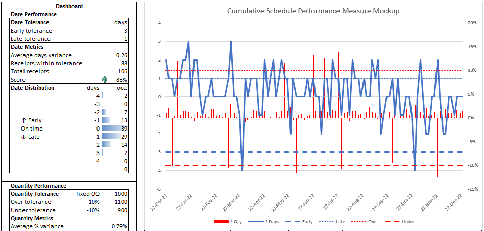
This chart incorporates three columns each for date and quantity: the variance, upper tolerance line and lower tolerance line. To add tolerance lines, columns are added to the data range, such as =SEQUENCE(106,,tolE,0), etc. Date variables are on the left axis, quantity variables are on the right axis. These six columns are initially assigned six colors, then changed to just two colors for clarity. The variances are solid, line for date and column for quantity; upper limits are dotted lines, lower limits are dashed lines. Thus, a manager can at a glance interpret a lot of information, identify outliers and trends, and investigate causes and interventions.

The Dashboard

The dashboard compiles and summarizes the metrics. In this example, date and quantity are separate sections. In each section, tolerances are given; metrics are listed, including average variance, receipts in tolerance (hits), total receipts, and % score; and a variance histogram is given.
Histogram
The histogram is created by two arrays, the bins and the occurrences.
The days bins adjust to the tolerance range: D13=SEQUENCE(
2*MAX(ABS(tolE),tolL)+3,,tolE-1)
The occurrences of date variances in each bin: F13=FREQUENCY(M4#,D13#)
The quantity bins and occurrences:
D34=SEQUENCE(7,,-0.15,0.05)
F34=FREQUENCY(W4#,D34#)
Occurrences arrays are given data bar format to present the familiar histogram appearance.
Metrics
I did not calculate hits in the data, so I'll use the histogram to count hits. First, I need to expand the bins array to be equal size to the occurrence array. I do this in a hidden column:
E13=EXPAND(D13#,ROWS(F13#),,MAX(D13#)+1)
This expanded bins range is now used to calculate hits:
F9=SUMIFS(F13#,E13#,">="&tolE,E13#,"<="&tolL)
Total records:
F10=SUM(F13#)
Score:
F11=F9/F10, with 5-colored-arrows icon set format
Likewise for quantity.
Conclusion
Metrics are often perceived by managers as a black box when they don't understand the process and mistrust their accuracy and accountability. It is surprising how often time and money spent on measures continue with no return. Simplicity and transparency are essential to success.
For small business, Excel may be the end state. For large concerns, it offers a way to simulate approaches that can lead to significant improvements.
Comments